Causation Probability Modelling

Introduction

A comprehensive collection of causation probabilities have been proposed in literature.

A risk model that may be used for evaluating the causation probability is presented further down this page. Inadequacies of a frequently cited risk model are discussed and instead we propose to apply Bayesian Networks. A Bayesian Network for obtaining the causation factor for ship-ship collision is established, and the results are compared to available statistics, where good agreement was found.

It is virtually impossible to formulate a full risk analysis that properly takes all relevant aspects into account. The modelling should, however, account for a subset as large as possible of the potential error mechanisms. This page describes the traditional risk analytical approach for obtaining the causation probability. We discuss the drawbacks of the traditional formulation and suggest applying Bayesian Network.

The subsequent Chapter 6 describes aspects that should be considered in the modelling.

Traditional Approach

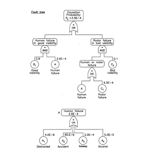
The traditional approach for calculation of Pc (i.e. analysing the cause leading to human inaction or external failures) is to formulate a fault tree or an event tree analysis, see Haugen [13], as shown in Figure 13.

Figure 13 Fault tree for causation probability Pc for collision against fixed object.

From this fault tree it is found that the causation probability Pc can be expressed as:

By application of such fault tree analyses for estimation of the causation probability, it is possible to examine the beneficial effect of new bridge procedures, of having a pilot on board, or of introducing a VTS system in certain geographical areas. Olsen et al. [22] studied the effect of a VTS system by an event tree analysis, see Section 6.2.1.

When inspecting the above fault tree it is questionable whether the modelling actually captures any of the important failure mechanism relevant for the considered critical situation. Factors that relate to navigational complications are not included in the analysis, although these are of importance for the relevant set of human errors. Moreover, it is seen that human failure contributes with 75% (2.6⋅10-4) to the causation probability. The dominance of the human failure is in agreement with observations.

However, the "Asleep" node is the dominant contributor (2.0⋅10-4) and it accounts for 60% of the causation probability. Although the dominating cause may be attributed to human errors this does not seem to be correct as high vigilance is expected in confined navigational areas. An important concern of the fault tree modelling is that the human factor model does not capture the relevant tasks that must be considered in the considered critical situation.

Using Bayesian Networks

Most practical risk analysis problems are characterised by a large set of interrelated uncertain quantities and alternatives. Within the conventional risk analysis different methods such as fault tree analysis and event tree analysis have been developed to address these problems. A fault tree analysis seeks the causes of a given event, and an event tree analysis seeks the consequences of a given event.

The two analysis techniques are supplementary methods, and when applied correctly the formulated model may reveal the entire probability structure of the model. Both fault tree analysis and event tree analysis – applied separately and combined – have in the past with success been used in the evaluation of the risk of various hazardous activities.

Unfortunately, both fault tree and event tree analyses do have their drawbacks.

• Firstly, it is difficult to include conditional dependencies and mutually exclusive events in a fault tree analysis (a conditional dependency is, for example, the dependence of the visibility on the weather; mutually exclusive events are, for example, good weather and storm). If conditional dependencies and mutually exclusive events are included in a fault tree analysis the implementation and the pursuing analysis must be performed with utmost care.

• Secondly, the size of an event tree increases exponentially in the number of variables.

• Thirdly, if the analysis should capture the primary failure mechanism, the global model, which is combined fault trees and event trees, generally becomes so big that it is virtually impossible for third parties (and sometimes even for first parties) to validate the model.

Here we advocate for using Bayesian Networks as the risk modelling and analysis tool.

A Bayesian Network is a graphical representation of uncertain quantities (and decisions) that explicitly reveals the probabilistic dependence between the set of variables and the flow of information in the model. A Bayesian Network is designed as a knowledge representation of the considered problem and may therefore be considered as the proper vehicle to bridge the gap between analysis and formulation.

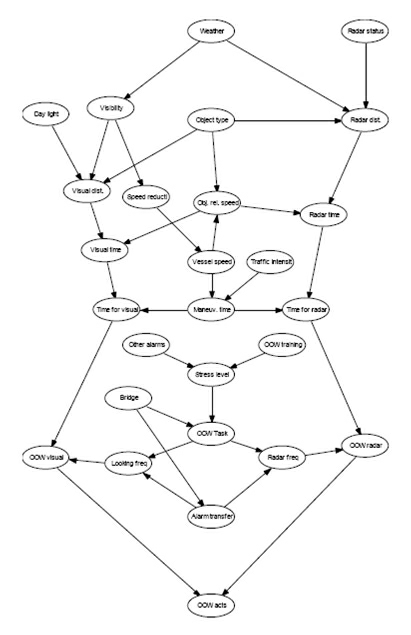
Figure 14 Example for Bayesian Network for a navigating officer reacts in the event of being on collision course with an object, from Friis Hansen and Pedersen [10].

A Bayesian Network is a network with directed arcs and no cycles. The nodes (to which the arcs point) represent random variables and decisions. Arcs into random variables indicate probabilistic dependence, while arcs into decisions specify the information available at the time of the decision. As an example, one node in the network may represent the weather, whereas another may represent the visibility. An arc from weather to visibility indicates that visibility is conditionally dependent on weather; see Figure 14.

The diagram is compact and intuitive, emphasising the relationship among the variables, and yet it represents a complete probabilistic description of the problem. For example, it is easy to convert any event tree or fault tree into a Bayesian Network. Conversely, it may not always be an easy task to convert a Bayesian Network into a combined fault tree and event tree, although theoretically possible.

A drawback of Bayesian Network is that they require the state space of the random variables (the nodes) to be defined as discrete states. In our above-mentioned example of weather and visibility, the state space of weather may easily be discretised into states as good weather, storm, etc., whereas the state for visibility more naturally would have been defined as a continuous state space. The Bayesian Network modelling does, unfortunately, require the state space of visibility to be discretised in ranges as for example, 0 to 1 km, 1 to 2 km, etc.

Although this is mentioned as a drawback, neither fault trees nor event trees offer any better alternatives. A consequence of the discretisation is partly that the result of the Bayesian Network may be sensitive to the selected discretisation, and partly that the calculations involved in the evaluation of the Bayesian Network grow almost exponentially in the number of states of the nodes. The latter is a consequence of Bayesian Networks encodes the entire probabilistic structure of the problem.

A focus on the causal relationship among the variables most effectively does the building of a Bayesian Network. This implies that a Bayesian Network becomes a reasonably realistic model of the problem domain, which is useful when we try to get an understanding about a problem domain. In addition, knowledge of causal relationships allows us to make predictions in the presence of interventions. Last, but not least, the model building through causal relationship makes it much easier to validate and convey the model to third parties. We will not give any details here on how Bayesian Networks are analysed. Instead reference is left to Jensen [18] and Pearl [23].

The Bayesian Network described above is taken from Friis Hansen and Pedersen [10] where a comparative risk evaluation of traditional watch keeping and one-watch keeping has taken pace. The results of the modelling were compared to observations, and good agreement was obtained. Here we extend the modelling to also cover ship-ship collisions.

Bayesian Network for Ship-Ship Collisions

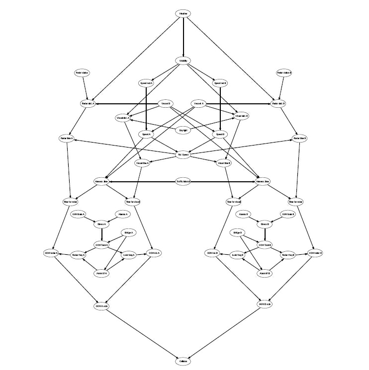
The network for predicting the causation factor for ship-ship collisions is rooted in the network shown in Figure 14. The Bayesian Network was extended to model two ships, i.e. ship-ship collision situations. The network used for this analysis is presented as Figure 15. It is seen that this Bayesian Network take into account the correlation between the two vessels, that is, they have to detect each other under the same conditions.

Although the network appears complicated, the elements from the basic network in Figure 14 are recognised. It is noted that the to more isolated groups in the lower part of the network models the behaviour on the two bridges, whereas the central group in the upper part of the figure models the two vessel that the two vessels has to be detected by each other.

Figure 15 Bayesian Network model for ship-ship collisions accounting for the correlation between the two vessels.

That is a factor which is very close to the causation factor Pc = 9.00 10-5 calculated by the Bayesian Network procedure for conventional vessels operating in geographical areas where the frequency of visibility less than 1 km is 3%. The modelling illustrates that it indeed is possible to establish a realistic modelling of the causation probability.

Table 1 Causation factors determined by Bayesian Network

Table 1 shows the calculated causation factors for all the combinations of meetings between large vessels with conventional bridge layout and vessels equipped for sole look-out.

It is seen that the calculated causation factor for meetings between conventional vessels is found to be, [10], Pc = 9.00⋅10-5.

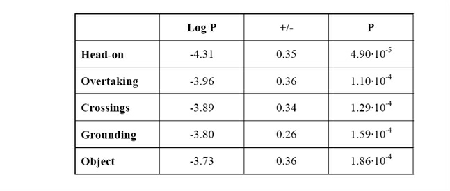
Table 2 Causation Probabilities from Fujii and Mizuki’s observations, Ref. [9].

This value can be compared with observed causation probabilities determined from large data sets published by Fujii et al. [9]. These observed values are given in Table 2.

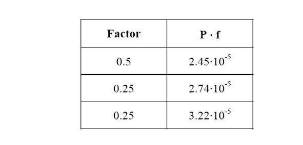
Table 3 Weighing Factors for headings:

In Table 3 the different headings have been weighed to obtain one global causation factor. The result is that the observations indicate that the causation factor is close to Pc = 8.41⋅10-5